Shortest version
Below I report my findings from a study I did on the effect current-drive amplification on a large number of speaker drivers. The main finding: when a driver is current driven, its distortion is reduced to levels comparable to drivers that are 6 times more expensive!
Short version
A couple years ago I went down the “current drive” rabbit hole. I tried it on a few drivers, saw big changes in odd-order harmonics, and then asked myself:
Is this a real, broadly useful effect… or did I just get lucky with a few samples?
So I built a measurement workflow (hardware + software + protocol) and measured 31 drivers, each one twice:
- once with conventional voltage drive (VF / voltage feedback)
- once with current feedback (CF) (high output impedance, current-controlled behavior)
What I found
- In the 200 Hz–4 kHz band, many drivers showed a clear reduction in odd-order harmonic distortion on CF.
- Averaged across the dataset, I saw roughly ~11 dB lower H3 and ~5–7 dB lower H5 in that band (details below).
- To put that into “dollars,” I plotted distortion vs normalized price metric (price/weight), and fit trend lines. The CF trend shifts in a way that corresponds to roughly a ~6× price multiple in the regression analysis.
If you want all the details and plots:
1. Download the full technical report (PDF)
2. Inspect and compare all measurements interactively in browser
Full version
Back story (why I did this)
I first came across the idea through a paper and then Esa Meriläinen’s book. I tested current drive on a few drivers and saw significant changes in odd-order HD. That was exciting — enough that I started thinking about building a proper current-drive amplifier for my own projects.
But building hardware is a big effort, so before committing, I wanted evidence that the effect is common across drivers, not a niche corner case. That’s what this dataset is: a “does this generalize?” check.
This took months longer than expected. If you’ve ever tried to get consistent/repeatable distortion measurements in a non-anechoic environment without a Klippel… you can probably guess why.
What is “current feedback” ?
Voltage feedback (VF) / voltage control
The amplifier tries to make the output voltage follow the input signal.
Current feedback (CF) / current control
The amplifier uses a feedback path that makes the delivered current behave more linearly, so nonlinear back-EMF of the driver is less able to turn into nonlinear current (and therefore nonlinear force).
This isn’t “EQ.” EQ can fix response shape; it doesn’t directly target the electrical/mechanical nonlinearity mechanisms that create harmonic distortion.
Measurement method
I don’t have an anechoic room or a Klippel, so these measurements are very near-field. That means SPL at the mic is high, and microphone distortion becomes a real problem if you’re not careful.
- Microphone: after trying a bunch of mics, I settled on an NTi M2010 because it stayed clean enough at high SPL.
- Mounting: each driver was mounted on a 16×16 inch baffle
- Mic position: 1 inch from the baffle, centered on the driver
- Distortion measurement: exponential sweep / Farina method
- Automation: QA403 via its Python API + SciPy tooling for signal processing
Why the sweep is “pre-compensated”
To compare drivers more fairly, I pre-compensated the sweep so that the measured acoustic output at the mic is essentially flat from 200 Hz to 4 kHz at 105 ± 0.1 dB SPL.
105 dB at 1 inch is not a normal listening measurement geometry, but it roughly corresponds to ~82 dB at 1 meter for a single 6” driver in that band (very rough, but it keeps the level in a “normal listening” ballpark for this analysis).
A note on “fairness” across driver sizes
Yes, this deviates from typical speaker measurement practice. The justification is pragmatic:
- Small drivers aren’t expected to compete with large drivers at far-field SPL.
- By measuring near-field and controlling level in the analysis band, I’m trying to compare motor distortion behavior at an output level that is more representative of what each driver might be used for, rather than “who wins at 1 m at the same SPL.”
It’s not perfect, but it gives a consistent basis for a large sample comparison.
Drivers measured
| Brand | Models |
|---|---|
| Tang Band | W8-1808, W4-1757SB, W4-1720, W3-881SJ |
| Purifi | PTT4.0X |
| Fostex | FF105WK, FE126En |
| Visaton | B100, GF200, B200 |
| SB Acoustics | SB20FRPC30-8, SB20PFCR30-8, SB12NRX, SB12PAC25-4, SB12PFC25-4 |
| Vifa | NE95W-04 |
| Fountek | FR88EX, FR88, FW135F, FW100B |
| Peerless | TC9FD-18-08, TG9FD10-04, 830656 |
| Seas | MU10RB-SL |
| Dayton | RS100-8, LW150, RS125S-8 |
| FaitalPro | 6FE100 |
| Polk | T15 5” woofer |
| Klipsch | Quintet 3” midwoofer |
| Wave Core | WF090WA01-01 |
| Multicomp Pro | 55-5650, 55-5670 |
The amplifier used
A TI TPA3255 amplifier board (BTL, with post-filter feedback) drove the drivers.
- One channel remained conventional (VF).
- The other channel was modified to incorporate current feedback.
- The CF channel achieved an output impedance of about 60 Ω and transconductance of about 1.75 A/V.
Each driver was measured once on VF and once on CF.
Results (the “6×” plot)
Most people (including me) find “11 dB lower H3” hard to interpret in terms of real-world value. So I tried a crude but useful translation: relate distortion performance to price.
What is “normalized price”?
I used a rough normalization to reduce “bigger drivers cost more” as a confounder:
- normalized price = price / weight
- then I express it as a multiple of the cheapest driver in the dataset
- the x-axis is log scale, so distance corresponds to price multiples
Yes — dividing by weight is crude. But it’s good enough to reveal a clear trend: more expensive drivers tend to have lower distortion (thankfully).
How to read the plot
- Blue dots: each driver measured on VF
- Orange dots: the same driver measured on CF
- Arrows connect the pair
- Blue/orange lines are best-fit regression trends (shaded region indicates uncertainty)
Reading tip: right = more expensive, down = lower distortion (better). Also, on this axis, a major step to the right is a 10× increase in normalized price.
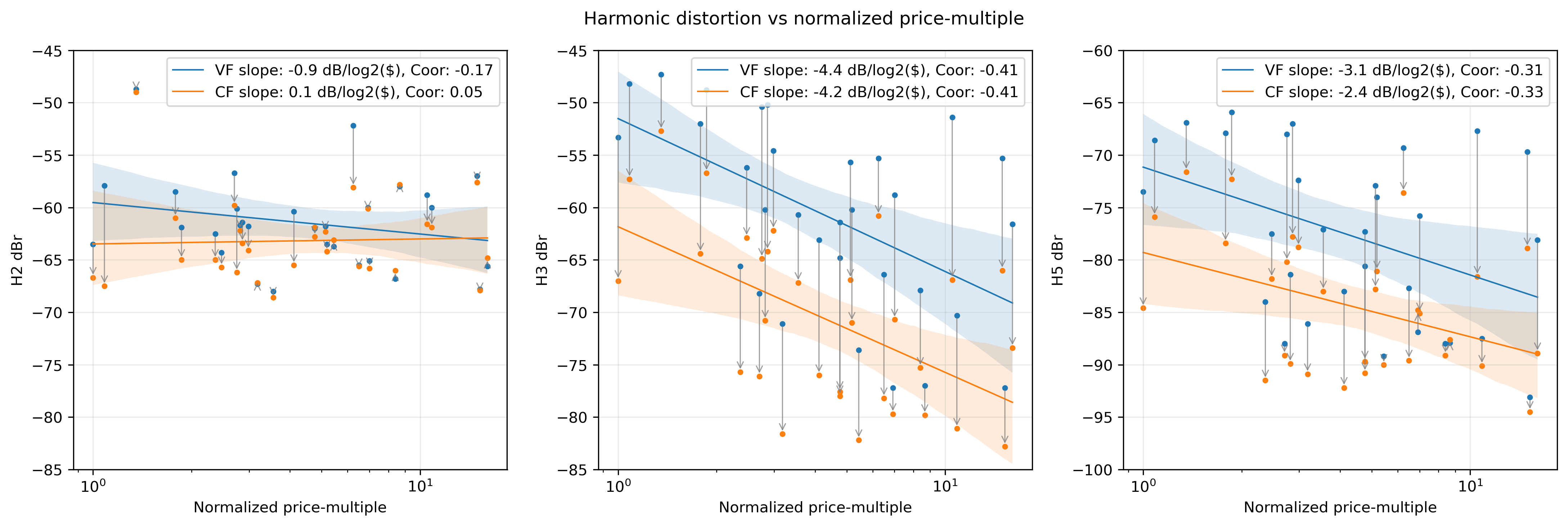 Harmonic distortion vs normalized price-multiple (31 drivers). Blue = voltage feedback (VF). Orange = the same drivers measured under current feedback (CF). Trend lines show the overall relationship.
The “6×” takeaway
The interesting part is the horizontal distance between the VF and CF trend lines. In the regression analysis, that shift corresponds to roughly a ~6× price multiple for odd-order distortion performance.
Put less formally:
On average, a driver on CF tends to land near the odd-order distortion performance you’d normally associate with much pricier drivers (by this normalized-price metric).
We could also look at how far the best fit line has shifted down. Across the dataset, in 200 Hz–4 kHz, CF reduced:
- H3 (3rd harmonic): ~11 dB lower on average
- H5 (5th harmonic): ~6 dB lower on average
Visual summary
If you want the “one glance” view, the plot below shows how much the harmonic distortions chnaged (relative to voltage drive) over the measured band.
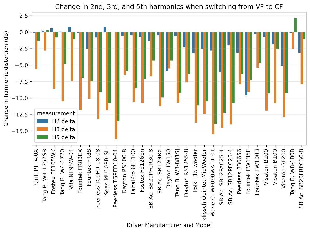 Relative change in harmonic distortion when switching from VF to CF (negative values indicate a reduction).
Limitations / notes
A few important caveats:
- This is one measurement protocol, one baffle, one microphone placement, one test level.
- Not all drivers in the study are intended to run cleanly to up 4 kHz (e.g. larger woofers) or down to 200 Hz (e.g. small midranges)
- Normalized price (price/weight) is a blunt instrument — useful for trend-spotting, not a law of nature.
If you’re the type who wants every detail, all of it is in the PDF:
Download the technical report (PDF)
Replication
If you’d like to replicate or extend this measurement set, I’m putting together a short “how I did it” guide (QA403 automation + sweep pre-compensation + analysis scripts).